This experiment has dual objectives. First, it is a classic experiment in characterizing the dynamic response of a system. In this case the response is a simple structure, described by theoretical methods of the type you have  studied previously in mechanics of materials, vibration and controls courses. Second, this experiment involves a typical application of analogue electronic instrumentation. It is also an experiment that is well suited to digital measurement, analysis and control.

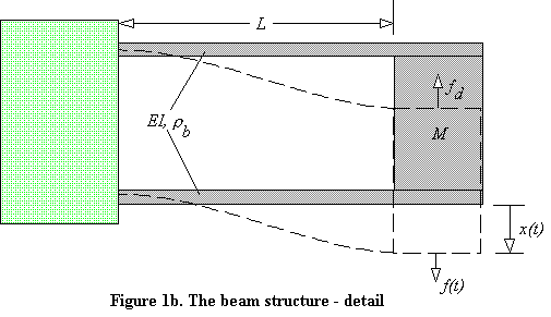
The following notation defines the properties of this structure:

• L = beam length
• EI = product of elastic modulus and beam area moment of inertia = beam bending stiffness
• k_b = effective spring stiffness of one beam of length L
• r_b = mass per unit length of one beam
• m = effective fraction of beam mass
• M = mass value of the rigid mass, including the mass value of everything rigidly connected to the mass (hardware clamping the beams to the mass, portions of the beams clamped to the mass, force coil, dashpot piston, and adapter blocks)
• b = viscous damping constant representing the dashpot's viscous action and the structure's inherent damping

The equation for k_b can be obtained directly from the standard beam element stiffness matrix (Megson, p. 458), or by applying the method described in Section 8.4 of Beer and Johnston. The value for m is an accurate approximation derived from advanced beam theory (Meirovitch, pp. 309-310). Since beam mass is small compared with M in this experiment, the value of m will have only a small effect.

We can now write the equation of motion for the laboratory structure. As a simple linear system, the equation of motion of the mass, under the action of a fluctuating force f(t) should be:

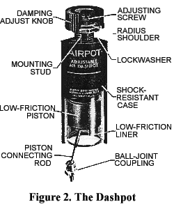
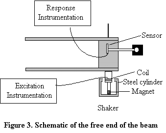
where, in this case, the total mass m will be the sum of the rigid mass and the contributions from the two beams (m=M + 2mr_bL), the total damping b will be that due to the dashpot plus that inherent in the system, and the total spring constant k will be the sum of the constants for the two beams (k=2k_b). Note that the representation of damping in Equation 1 is approximate, since it assumes ideal viscous damping (force proportional to velocity). The inherent damping of this laboratory structure is very small, so that almost all of the damping you will observe is caused by the dashpot ( figure 2). In the experiment an electromechanical shaker will be used to exert a sinusoidal excitation force f(t) onto the mass at the end of the beam, as shown in figure 3.  A proximitor (a non-contact position sensor) will be available to measure the resulting translation of the mass x(t), as also shown in figure 3.

Solution to the equation of motion for sinusoidal fluctuations.
The behavior of the structure, characterized by the relationship between forcing f(t) and the displacement it produces x(t), is of course given by the solution to equation (1). One way to obtain this is by Laplace transform (see Ogata, example 7-2). An alternative route, that explicitly recognizes our interest in the response of the structure to different frequencies of forcing, is to assume a sinusoidally fluctuating force and (since the system is linear) a corresponding sinusoidally fluctuating response. Adding a fictitious imaginary part we write

where w is the angular frequency of the sinusoidal fluctuation. F(w) and X(w) are complex numbers whose magnitude represents the amplitude of the force or displacement fluctuation, and whose argument (angle) represents the phase of that fluctuation. We note that,

Substituting into equation 1 we thus obtain

Canceling e^jwt we obtain,

and thus

…………..(2)

So, the ratio between the amplitude of the displacement x_m and the amplitude of the force that produces it f_m at angular frequency w is

………….(3)

referred to as the dynamic flexibility. The phase lag y_m between the displacement fluctuations and the force fluctuations producing them at angular frequency w is

…………(4)

We can summarize these results as indicating that, with the mass excited by a sinusoidal force f(t)=f_msin(wt), the solution for the steady-state sinusoidal displacement of the mass is x(t)=x_msin(wt+y).   It is worth making some observations here:

a)      The dynamic flexibility (equation 3) at zero or very low frequency is simply 1/k. This is termed the static flexibility.

b)      If the system were undamped (b=0), the dynamic flexibility, equation 3,  would become infinite when k=mw ², in other words when the frequency . This is termed the natural frequency of the system and given the symbol w_n.

c)      The dynamic flexibility peaks when the denominator of equation 3 is at a minimum. This condition is called resonance. The resonant frequency is close to the natural frequency for light damping.

d)      At the natural frequency the phase response of the actual damped system (b>0), is -90 degrees, regardless of the damping.

e)      At the natural frequency the dynamic flexibility of the actual damped system is given by . Dividing this by the static flexibility 1/k we obtain a ratio of . This defines the parameter z, referred to as the viscous damping factor.

f)        At frequencies much larger than the natural frequency the dynamic flexibility varies as 1/(mw ²), and the phase response as tany_m =b/(mw). Thus, when plotted on a log-log scale the dynamic flexibility tends to slope of -2 at high frequency, and tany_m  tends to a slope of -1.

g)      At frequencies well below the natural frequency, the phase (in radians) varies with frequency linearly, as tany_m =-bw/k.

h)      The phase is always between 0 and -p.

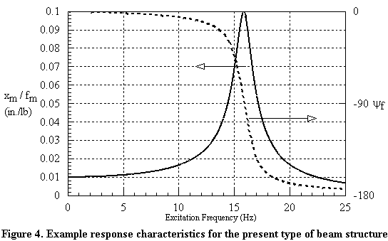
The above analysis suggests a straightforward procedure for experimentally determining the dynamic response of a structure, and the parameters that characterize it. We simply provide a force to our structure that varies sinusoidally at a particular frequency w with a defined (or measured) amplitude f_m. We then measure the steady state amplitude of the displacement fluctuations that force produces x_m and the phase lag between the excitation and response y_m. This is then repeated for a range of frequencies. In the process we can discover the point where the phase lag reaches -90 degrees (the natural frequency) and the amplitude response is at a maximum (the resonant frequency), the phase and amplitude variations at low and high frequency, as well as the overall form of the response. It is exactly this type of scheme you can implement using the analogue instrumentation available with this experiment.

1. Measure the dynamic flexibility at very low frequency to get k. (You may want to measure at two very low frequencies to see if the values of k are consistent and thus the frequency low enough.)
2. Measure the natural frequency using the phase lag. Using the value of k we already have, this will give m.
3. Measure the dynamic flexibility at the natural frequency and use that (along with the values of k and m already estimated) to get b.

Think up some schemes for yourself.

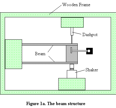
The apparatus for this experiment can be described in three different groups, as suggested by figure 3 : the structure, the excitation system, and the response system. Note that the excitation and response systems use much of the electronic instrumentation you have already been introduced to in instrumentation lab.

A. Beam Structure, General Items
The beam structure should be are mounted on the lab floor. (Unlike a desk, for example, the lab floor won't vibrate significantly and thus become part of the dynamic system). The following are its nominal characteristics:

Weights that may be added to the mass (in the form of large steel washers) are available. Calipers, a steel ruler, a tape measure and digital scales are available for you to record/check all dimensions/weights as you feel appropriate.

A digital camera will be available for you to record picture of apparatus and instrumentation.

The structure is provided with the excitation and response systems described below.

B. Excitation System
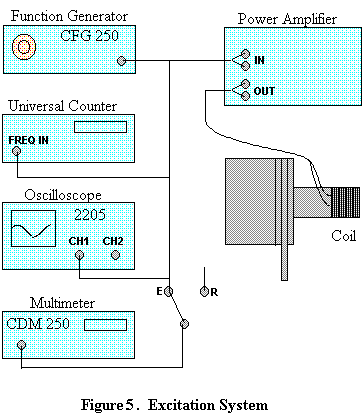
Figure 5 is a functional diagram of the excitation system. The purpose of the excitation system is to produce and measure the sinusoidally fluctuating force f(t) = f_msin(wt) used to shake the structure.
A Tektronix CFG250 Function Generator is provided to produce the sinusoidal excitation signal. This is the same instrument you have already been introduced to in Instrumentation Lab. The generator should be set up to produce a sine wave in the 10 Hz range with an amplitude of less than 2V. Remember that the sine wave will be produced at the 'Main' output socket.

To accurately measure the frequency or period of this signal (an important parameter, see equations 1 or 2), a  Beckman UC10A Universal Counter is provided. The UC10A is more suitable for the low frequency signals (<20Hz) used in this experiment than Tektronix counter you have met previously. In particular, it can display the period of the sinusoid to three or four significant digits. Examine the UC10A, and have the instructor explain how to use it.

A Tektronix 2205 Oscilloscope is provided to display the excitation signal, and a Tektronix CDM250 Multimeter to display its  root-mean-square (RMS) voltage.  Both the oscilloscope and the multimeter provide a means to measure the voltage amplitude (recall that the RMS is 0.7071 of the amplitude) and thus, indirectly, the force amplitude f_m applied by the electromechanical shaker. (However, note that the multimeter is not accurate for this purpose below about 10Hz). The shaker itself requires a relatively large current, and thus cannot be driven by the voltage signal of the function generator itself. Instead, the connection is made through a power amplifier, which outputs a current that follows the excitation voltage. The sinusoidally fluctuating current drives the electrical coil of the shaker. The coil lies in the field of a permanent magnet contained in the steel cylinder, and thus the current results in the generation of an electromagnetic force. Figure 6 shows the coil calibration, in pounds force produced per volt of excitation. As you can see the calibration is close to 0.0817 lb/volt, with a very slight variation with position.

The power amplifier and shaker are already connected. BNC cables and connectors are provided to connect the rest of the excitation system.

C. Response System
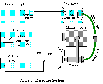
Figure 7 is a functional diagram of the response system. The purpose of the response system is to sense and measure the displacement of the structure x(t) = x_msin(wt+y)  in response to the sinusoidal load.

The fluctuating position of the mass is measured using a non-contact device known as a proximitor that uses radio frequency waves and a steel target. The proximitor system is manufactured by the Bentley Nevada Corporation and consists of a probe, type 300-00-00-30-36-02, and a proximitor, type 3120-8400-300, and a Tektronix CPS250 power supply. When connected as shown in Figure 7, this sensor detects the gap between the probe tip and a steel target attached to the laboratory structure.

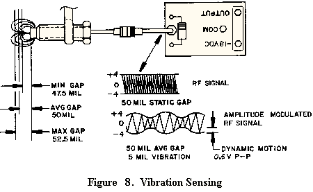
The proximitor converts the -18 volts from the power supply into a radio frequency (RF) signal that is applied to the probe through cables. A coil within the probe tip radiates the RF signal into the surrounding area as a magnetic field (see figure 8). If there is no electrically conductive material (such as the steel target) close enough to intercept the magnetic field, then there is no power loss in the RF signal, and the voltage at the proximitor output terminal is maximum (about -14 volts). If a conductive target is close enough to the probe tip to intercept the magnetic field, then eddy currents are generated on the surface of the material, resulting in a power loss in the RF signal, and the negative voltage at the output terminal is reduced.  If the conductive surface comes very close to the probe tip, then all of the RF power is absorbed, and the output voltage reduces to zero.

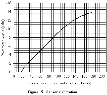
For a certain range of separations between the probe and the target, there is a linear relationship between gap and output voltage. Figure 9 is the calibration curve for the particular sensor used in this experiment with its steel target. The linear range is between an output voltage of -1.5 and -9.5 volts, corresponding to a gap of between 25 and 100mils (0.025 to 0.1 inches). In this range the sensitivity of the proximitor is close to 106 millivolts/mil. In otherwords, a vibration of the beam with an amplitude of one thousandth of an inch would produce a fluctuating voltage signal from the proximitor output with an amplitude of 0.106V. Alternatively, if you measure a 1V amplitude signal from the proximitor, that indicates an amplitude of the beam motion x_m = 1/0.106 = 9.43 thousandths of an inch.

As sketched on figure 7, the probe is attached to an arm that extends from a magnetic base. The base is clamped magnetically to a steel plate that is screwed to the wooden frame. The magnetic field of the base can be turned on or off with a large switch in the base, so the switch essentially attaches the base to or releases it from the steel plate. The probe tip must be positioned initially a certain gap distance away from the center of the steel target, as shown on figure 7, and the face of the probe tip should be approximately parallel to the target surface (in other words, the axis of the probe should be perpendicular to the target surface). There are adjustment knobs on the arm connecting the probe to the magnetic base, but you should avoid using these if possible. The best way to position the probe relative to the target is to switch off the magnetic field of the base, then gently slide the magnetic base on the steel plate until you get the correct positioning, then switch on the magnetic base to clamp the entire assembly in the correct position.

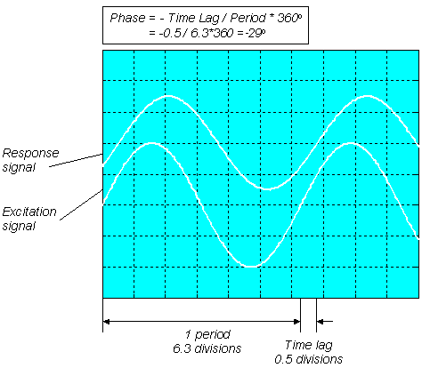
As shown on figure 7, the proximitor output voltage is connected for observation and data recording to channel 2 of the Tektronix oscilloscope and to the Tektronix voltmeter mentioned in the excitation section. Since the oscilloscope can display both the excitation and response signals simultaneously, it can be used to measure the phase response y.  Figure 10 shows an example of how this can be done. Notice how both signals have been positioned symmetrically around a horizontal grid line, making it easier to see the time delay between the two signals as a time between two zero crossings.

This technique is fine in general (you can probably use the figure here to make an estimate of its likely accuracy), but there is a much quicker way of using the scope to tell when  the phase lag is exactly 90^o and thus determining when the system is being excited at its natural frequency. The technique is to use the X-Y capability of the scope, to plot the excitation signal against the response signal in what is called a Lissajous figure. The following links are movies that show examples of Lissajous figures produced for phase angles of 0 , -45 , -75 , -85 , -90 , -95 , -115 , -135 and -180 degrees. The elliptical figure in the top right hand corner of  each movie shows what you would see on the scope for the phase angle indicated with the excitation signal connected to channel 1 of the scope (X) and the response to channel 2 (Y).

Note that only when the phase is exactly -90^o  are the major and minor axes of the Lissajous figure exactly vertical and horizontal. You may be able to use these movies, with some actual scope experience later to estimate the error in the phase angle, measured using this technique. The Lissajous figure is by far the quickest way of determining the natural frequency of a system, or the change in the natural frequency when the system is altered.

A. Getting familiar with the equipment
The following procedures are designed to help you get a feel for the beam structure and its instrumentation. It is important that you get a hands-on feel of how to use the apparatus and what its capabilities and problems are. Feel free to play with the apparatus (but see item 2 concerning the power amplifier first). Don't forget to record any results, thoughts, ideas, plans, photos or concerns in the logbook.

• Begin with all the electrical items turned off. Turn on all components of the system except the power amplifier. Adjust the function generator to produce a sine wave of about 10 Hz. Play around (ask the instructor, look at the instrument) until you have set up the counter to display the period of this sine wave to at least 3 digits, and then set up the scope to show this signal on channel 1. Try changing the settings on the scope. Try adjusting the volts/div. Set the vertical position to place the trace symmetrically about a horizontal graduation, as in figure 10 . Look at the multimeter. Read the RMS voltage. Check to see if the RMS is consistent with the amplitude shown on the scope (check the relationship between RMS and amplitude). If not, make sure the small knob at the center of the VOLTS/DIV control on the scope is set to 'CAL'. Decide whether you will rely on the scope or RMS meter for your amplitude measurements, and estimate the accuracy of the method you select. It would be a good idea to record your choice, your reasons and your accuracy estimate in the logbook.
• Be careful with the power amplifier as, through the shaker, it turns the electrical signal into a real world mechanical movement. While a 10V excitation amplitude may look innocuous enough on the scope, turn on the power amplifier and, as the shaker system blows up, the beam may break the proximitor. (On the other hand, what's the loss of a proximitor after the loss of an eye from an exploding coil). So, before turning on the power amplifier, turn down the amplitude on the function generator to zero. Then turn on the power amplifier. Increase the amplitude slowly until the beam begins to vibrate slightly (an amplitude of 2V may be about right). If it doesn't start to vibrate, lower the amplitude, turn off the power amplifier and check the circuit. If it does, look at the excitation amplitude on the scope, and the RMS amplitude on the multimeter. Practice figuring out what force amplitude is being applied to the beam. Turn down the amplitude and switch off the power amplifier.
• Now turn your attention to the response system. Investigate the proximitor. Switch the response system on, including the proximitor power supply. Set the multimeter to read the DC voltage coming from the proximitor output (previously you had it set to AC to measure the RMS excitation signal). Now, use one of the adjustment knobs on the proximitor probe mount to move the probe back and forth from the target (you can also try releasing the magnetic base and moving the whole assembly around). As you move the probe, watch the voltage. Does it change? how much? is the size of the change roughly consistent with the amount you are moving it, given the calibrated sensitivity (see above). Discuss how far you should set the proximitor from the target with the beam not moving, if you want it to operate in the linear range of its calibration (figure 9 ) when the beam is vibrating. Set the proximitor in this position using the DC output voltage as a guide.
• Investigate the scope. Check the function generator amplitude is still turned down. Turn the power amplifier back on and get the beam vibrating again. Adjust the scope so you can see both excitation and response, as in figure 10 . Practice determining the phase lag from the scope screen. (If one of the signals is inverted, use the CH2 INVERT switch to get them the same way up). Practice determining the amplitude of the beam motion x_m (in inches) from the signal on the scope screen, and then practice getting it from the multimeter (remembering the lower frequency limit on the multimeter). Choose your method of measuring dynamic flexibility, explaining the choice and estimated accuracy in the log book.
• Investigate the beam. Gently play with the amplitude of the excitation and see if you can observe the linearity of the relationship between excitation and response. Now, try slowly varying the frequency. If you were at about 10Hz, as you increase the frequency the response amplitude will get bigger. You want to counter this by lowering the amplitude of the excitation signal otherwise, sooner or later, the response will get so large that you will go beyond the linear range of the proximitor, and the range of motion of the beam. As the excitation signal appears smaller and smaller on the scope, you may want to change the VOLTS/DIV on that channel so you can easily see it, and its phase relationship with the response. Take the frequency up to get a feel for where the response is a maximum, and where the natural frequency is, at least roughly.
• Try the Lissajous. Set the scope to XY and look at the Lissajous figure. Adjust the VOLTS/DIV on the two channels to make a nice fat ellipse. Slowly adjust the frequency (again keep the response in check by adjusting the excitation amplitude) and watch the figure change. Note that, especially around resonance, it may take at least a few seconds for the beam (and thus the Lissajous figure) to settle down after you change the frequency. Does the figure behave correctly, given the expected change in phase with frequency? Can you find the natural frequency? Estimate how accurately you can determine the natural frequency with this method. While the beam is moving at the natural frequency, put one or two of the washer weights on it. Observe what happens to the Lissajous? Can you readjust to the new natural frequency? Why do the washers change the frequency? Might the digital weighing machine be of some use in predicting this effect theoretically? Think about it. Use the log book.
• Make a list of all the important parameters of the system that you can determine and may influence the system response, including dimensions.

Goal 1. Design, conduct, and implement a test or series of tests to estimate the three key parameters (total mass m, total damping b, total spring constant k) of the beam system using the scheme laid out at the end of section 2, 
Suggestions. It is really important to estimate the uncertainty in your results. You may be able to reduce this uncertainty by using extra measurements to get additional estimates, and averaging the answers. Keep careful documentation of what you do, why you do it, set up characteristics, expected results, unexpected results, analysis, photos and plots in the electronic log book as you proceed. Analysis as you go will help catch bad data or points before it's too late. It will be interesting to look at any differences between the your estimates the total mass and spring constant, and the nominal values that can be inferred from the information above. In assessing the significance of any differences measurements of the actual beam dimensions and imperfections may be useful.

Goal 2. Design, conduct, and implement a test, or series of tests, to investigate the extent to which the beam can be approximated as a linear system.
Suggestion.  Measuring the entire response (phase and dynamic flexibility) characteristic is not such a bad way to proceed, but you may wish to focus your measurements on characteristics/regions of the response that are particularly identifiable with a linear system. Of course your assessment of the degree of validity of the linear response model will have to factor in your estimates of the accuracy of your results (e.g. comparing phase response measurements with theoretical estimates on a graph won't mean much without error bars on the phase measurements, as you won't know if the differences are significant or not).  Plotting as you go will help catch bad data or points before it's too late. Keep careful documentation of what you do, why you do it, set up characteristics, expected results, unexpected results, analysis, photos and plots in the electronic log book as you proceed.

Goal 3. Design, conduct and implement a test, or series of tests, to document the dependence of the natural frequency on the total mass M of the system, and compare with linear theory.
Suggestion. Don't forget the washers.  The uncertainty on the natural frequency measurement, and on the original mass of the beam (and other factors) will be important factors if you really want to draw definitive conclusions from a comparison with the theory. Keep an eye out for un-controlled parameters or beam behavior. Plotting/analysis as you go will help catch bad data or points before its too late. Keep careful documentation of what you do, why you do it, set up characteristics, expected results, unexpected results, analysis, photos and plots in the electronic log book as you proceed.

1. Beer, F. P. and Johnston, E. R., Mechanics of Materials, 2 ^nd ed., McGraw-Hill, 1992.
2. Megson, T. H. G., Aircraft Structures for Engineering Students , Wileyl (Halsted Press), 1990.
3. Meirovitch, L., Elements of Vibration Analysis, 2^nd ed., McGraw-Hill, 1986.
4. Ogata, K., System Dynamics, 3^rd ed., Prentice Hall, 1998.