You will be given further specific instructions during lab. Copies of any materials will be made available on this page, linked from the left hand column). The material below gives a complete description of the techniques you will be using in lab.
 

Consider a signal generated by a probe (such as a hot-wire anemometer) sensing the velocity in the wake of a circular cylinder. The velocity fluctuates with time because the flow is unsteady. 

Imagine you are measuring this signal as part of an experiment to understand the flow and its effects. The portion of the velocity signal shown clearly contains important frequency information. We see fluctuations at several frequencies apparently connected to the passage of eddies over the probe and the frequency at which eddies are shed from the cylinder. If the cylinder were supported by a flexible structure, knowing this shedding frequency would tell us the frequency at which that structure would be excited and thus its the structural response. So this information is clearly valuable for several reasons, but how do we get it? How do we determine what frequencies are in the signal?

When a signal contains only one frequency (i.e. it is sinusoidal) determining that frequency, its amplitude and phase can be a straightforward process (we discuss one such method at the end of this chapter). However, real signals are usually not sinusoidal, contain many frequencies and may contain random elements. Determining the frequency content of such a signal requires more sophisticated methods, referred to collectively as spectral analysis. The primary purpose of this chapter is to explain the methods of spectral analysis, their usage, capabilities and limitations.

Consider the general expression for a sinusoid, using the cosine function.

The function has a frequency f (in Hertz) that is equal to the inverse of the time it takes to complete one period of oscillation. At a given frequency it takes two pieces of information to specify such a wave; its amplitude A and its phase e. Note that the amplitude is half the peak to peak fluctuation and, if you work it out, the r.m.s. is 1/Ö2 = 0.7071 of the amplitude. Note that the phase is an angle, and that negative phase corresponds to positive time delay of the wave.

When we ask the question "what frequencies are in the signal?" what we really mean is "If we fit the shape of the signal to a sum of sinusoids of different frequencies, what is the distribution of amplitudes and phases as a function of the frequency?" This question has a useful answer because of Fourier's theorem which states that any signal of zero mean value can be represented as a unique sum of sinusoids.

When we decompose our signal into its component sinusoids, the resulting plot representing amplitude or phase as a function of frequency is referred to as a spectrum. There are three types of spectra we need to be concerned with at this stage:

1. The amplitude spectrum. A plot of the sine wave amplitude vs. frequency. Note that when engineers refer to the amplitude spectrum they may either mean the amplitude itself A or the r.m.s. amplitude (=0.7071A). You often have to look carefully (or ask) as to which is being used.

2. The phase spectrum. May be plotted in radians or degrees.

3. The power spectrum. A plot of Amplitude²/2 vs. Frequency.  This is called the power spectrum because the square of the variable represented by the amplitude (e.g. velocity, voltage, displacement) is often proportional to a rate of work being done. However, the term power spectrum always means Amplitude²/2 vs. Frequency even when this isn't the case.

The idea of obtaining a spectrum from a measurement may seem overwhelming, not least because signals in the natural world can contain infinitely many frequencies. However, such signals also contain infinitely many time steps and that doesn't stop us from measuring their behavior with time by sampling them at regular intervals over some limited time. In an exactly analogous way, measuring a spectrum is an exercise in sampling it at regular intervals in frequency over a limited frequency range. To understand how this comes about we need to consider the whole measurement process.

Consider once more the velocity signal from our cylinder wake. To measure this signal we take samples of it at regular intervals Dt. We already know that the maximum frequency we can observe in such a sampled signal is the Nyquist frequency, equal to half the sampling rate. Thus by sampling in time we already have set the maximum frequency we can measure as 1/(2Dt). (There may be problems, of course, if our original signal contains frequencies higher than this, so our measurement is aliased, but more about that later.)

Inevitably we can only take samples of the signal for a finite time called the total sampling time T. We refer to this process of extracting a finite length piece of the signal as windowing (the idea being that we are looking at the signal through a window in time). The lowest frequency we can unambiguously infer from a windowed signal is one with a period that lasts the total sampling time. Thus, if N is the number of samples we took, then the total sampling time T=NDt and the lowest frequency we can measure is 1/T=1/(NDt). Note that this also turns out to be the smallest difference in frequency we can infer from the windowed signal.

So when we sample the signal at time intervals of Dt over a total time T=NDt it turns out that we are also sampling its frequency content at intervals of 1/(NDt) up to a maximum frequency of 1/(2Dt).  As a practical example, if our velocity signal is being sampled at a rate of 10Hz (Dt=0.1s) and we are taking the 32 samples shown then we have sampled its frequency content at intervals of 0.31Hz=1/(32´0.1s) up to a maximum frequency of 5Hz=1/(2´0.1s).

Now consider the problem of calculating the spectrum, i.e. expressing our sampled signal as a sum of sinusoids each of different amplitude and phase. Since the sinusoids will have a maximum frequency of 1/(2Dt) and a frequency interval of 1/(NDt), we will have  1/(2Dt) ¸ 1/(NDt) = N/2 of them. This makes good mathematical sense. Since we need two pieces of information (amplitude and phase) to define each sinusoid, we will have N pieces of information to obtain using the N samples of the signal that we originally took. Obtaining the mathematical expressions for the amplitude and phase in terms of the original sampled values of the signal can thus be thought of as an exercise in solving N equations for N unknowns.  Performing the math, we find that the amplitude and phase of the nth sine wave, having a frequency f_n=n/(NDt), is:

where the coefficients a_n and b_n are given in terms of our original signal v(t) as:

Note that the index i in these expressions just references the samples that we took so, for example, i=3 references the third sample we measured v(3Dt). These expressions, for determining the amplitude and phase as a function of frequency, are referred to as the Discrete Fourier Transform. The discrete Fourier transform is closely related to the continuous Fourier transform used in analyzing linear systems and, for example, in controls and dynamic response problems. This close relationship makes the spectral analysis particularly useful when we use it in experiments that deal with such systems or problems. 

The expression for our original sampled signal in terms of the sum of these sinusoids is:

This expression (which effectively reverses the process of determining the amplitude and phase from v(t)) is referred to as the Inverse Discrete Fourier Transform. Note that it contains one extra coefficient A₀/2 that we didn't anticipate, apparently for zero frequency. Following through the expressions for a_n and b_n for n=0, however, you will find that this extra coefficient simply represents any mean value of the signal which cannot be accounted for in the sum of sinusoids.

The figure below shows spectra obtained by taking the discrete Fourier transform of our example velocity signal.

Note that the spectra are plotted against frequency index n, Interpreting these spectra is not hard if you remember the meaning of the frequency index n plotted on the horizontal axis. Specifically n=1 corresponds to a wave with a wavelength that fits one time into the sampling window, n=2 is a wave that fits twice into the sampling window, and so on. The power spectrum shows large amplitudes for waves that fit 3 and 6 times into the sampling window, with phases of about -40 and 45 degrees respectively. Look at the sampled and windowed signal and see if you can identify these components in the original data by eye. Confirm in your own mind that, for a 10Hz sampling rate, these peaks are occurring at frequencies of 0.94Hz and 1.88Hz.

Finally, note that the phase values only have meaning when the amplitude is non zero (a sine wave with zero amplitude looks the same whatever the phase is). Thus, in the present case, the phase values for frequency indices of 11 to 16 means little. 

In this, and the following section, we will look at some of the practical issues of computing spectra from a measured signal, with particular reference to LabView. We will examine a number of examples that involve LabView spectral analysis of sine-wave signals. We use these single frequency signals because they are easily understood and therefore reveal clearly both the capabilities and limitations of spectral analysis. However, don't forget that the real power of spectral analysis is that it can be applied to any signal, whatever form it has, and however many frequencies it contains.

While the above equations for computing the discrete Fourier transform and its inverse are entirely correct, they are rarely used explicitly. This is because they contain a lot of redundant arithmetic and so much faster algorithms for computing the same results are usually used. These are called the Fast Fourier Transform (FFT) and Inverse Fast Fourier Transform (IFFT). We won't describe these algorithms here and you don't need to consider programming them since they have been part of standard software packages ever since such packages have existed (an indication of how important and universal spectral analysis is). Such packages often scale and present FFT results differently, however, so it is important that you find out what your software does before you use it. Below we look at computing FFTs in Matlab and LabView.

4.1 Matlab
Suppose the original samples of our signal in an array v with elements 1 to N. The command c=fft(v); computes the fast Fourier transform of v and places it in the complex array c. To get the above coefficients from c we have to scale it and separate it into real and imaginary parts. We would write

a=real(2*i*c/N);
b=imag(2*i*c/N);

to get arrays a and b containing the coefficients a_n and b_n (where the nth array element corresponds to the nth coefficient).  Note that in Matlab i refers to the square root of -1. With the coefficients a_n and b_n it is a straightforward matter to go ahead and calculate the amplitudes and phases and plot their spectra.

Performing the inverse transform basically means reversing this process. Starting with arrays a and b containing the coefficients a_n and b_n we would write...

c=(a+i*b)*N/2/i;
v=ifft(c);       

...to recover the sampled time signal v. 

4.2 LabView
There are many LabView functions that deal with computing FFTs, spectra and related quantities. For now we will concern ourselves only with the 'Spectral Measurements' express VI. This computes the exact amplitude and phase values defined above explicitly. You can demonstrate this for yourself by writing a short LabView program, as follows.

1. Open a blank vi.

2. Right click on the empty block diagram and select 'Input' and then 'Simulate Sig'. This will add a VI that simulates the measurement of a signal.

3. Position the VI on the block diagram and a dialog box will open inviting you to set the characteristics of the measured signal. The default setting is for 100 samples at 1kHz of a 10.1Hz sine wave with an amplitude of 1 and phase of zero. This is fine, except for the frequency which you should change to 50Hz before clicking OK. Can you figure out what the frequency range and resolution for this signal will be?

4. Now, to take the FFT of this signal, right click again (on a blank space) and select 'Analysis' and then 'Spectral'. Position this VI and an second dialog will open, asking you to pick the details of the spectral analysis you want. Under 'Spectral Measurement' change the selections to 'Magnitude (Peak)' (LabView's terminology for an amplitude spectrum), and 'Linear' (so that LabView doesn't take the log of the results). Under 'Window' choose 'None' (more about this later).

5. Connect the 'Sine' output of the Simulate Signal VI to the 'Signals' input of the Spectral Measurements VI. This completes the computational part of the code.

6. To plot some results, go to the front panel and add three graphs (for each, right click, select 'Graph Inds' and then 'Graph') and arrange them as you like.

7. Back on the block diagram, connect the first graph to the 'Sine' output of the Simulate Signal VI, and the second and third graphs to the 'FFT-Peak' and 'Phase' outputs of the Spectral Measurements VI. Your code is now complete. The final block diagram should look like that below.

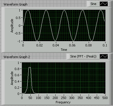
Now go to the front panel and hit the run button. After a brief delay the results should appear much as shown below. Note that, with the exception of the name on the vertical axis of the phase plot (which you may wish to type in manually - just click on it), the plot axes and labels should automatically label themselves to sensible things when you first hit the run button.

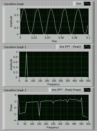
If you have trouble getting your code to run, you can download the version illustrated above, called spectralDemo.vi. You will see that the amplitude spectrum from the FFT shows a value of 1 right at 50Hz, and a phase of -1.57 radians (= -p/2 = -90 degrees) here. Everywhere else the amplitude is zero and the phase is meaningless (as discussed above).  Confirm in your own mind that you are happy with this result, i.e. that the signal in the first graph decomposes into just one cosine with an amplitude of 1 and a phase of -90 degrees.

Note that the Spectral Measurements VI is easily modified to output the spectra in any one of a number of standard forms. Double click on the Spectral Measurements VI to open the dialog and look at the options available. First, by checking the box on the lower left, you can change the output phase to be in degrees. Likewise, by changing the selection under 'Spectral Measurement' to 'Magnitude (RMS)', you can have the output amplitude spectrum multiplied by 1/Ö2 to indicate the r.m.s. values of the component sinusoids.

Alternatively you can also change the spectral measurement option to 'Power Spectrum' or 'Power Spectral Density', but be aware when you do this that the Spectral Measurements VI will lose the phase output, so you will have to delete the phase graph and clean up the wiring. Consistent with our definition above, the VI outputs spectral values equal to half the square of the amplitudes (½A_n²) when the power spectrum option is selected. The power spectral density is the same as the power spectrum, but with the values divided by the frequency resolution, i.e. ½A_n²(NDt). The power spectral density can be thought of as showing the 'power' per Hertz. This representation can be useful when measuring signals that contain a continuous distribution of frequencies. Such signals produce power spectral levels that depend on the frequency resolution implied by the windowing of the signal. Using the power spectral density avoids this problem.

The 'Spectral Measurement' portion of the dialog also allows you to change the result type from 'Linear' to 'dB'. With dB selected the VI outputs the spectral levels in terms of decibels. The term 'decibels' refers to a logarithmic scale, rather than a different set of units. Specifically, for quantities proportional to the amplitude, the level in decibels is 20log₁₀(quantity). For quantities proportional to the amplitude squared, the level in decibels is 10log₁₀(quantity). Thus selecting 'Magnitude (RMS)' and 'Power Spectrum' produces the same result in the amplitude spectrum when that result is presented in terms of dB.

4.3 Exercises using LabView
To perform these exercises you will need to download and open the code spectralDemo.vi.

1. Generate plots of the amplitude and phase spectrum of a 30Hz sine wave, with a phase of 45 degrees and an amplitude of 5, inferred from 100 samples of the signal measured at a rate of 1kHz. Plot the phase spectrum in degrees. Explain why the phase spectrum is not 45 degrees at 50Hz. Explain the significance of the phase spectrum at other frequencies.

2. For the sine wave in problem 1 replot, in linear form, the amplitude spectrum as an r.m.s. spectrum, a power spectrum, and as a power spectral density. Using the formulae given above show that values of each of these spectra at 30Hz are consistent with the original amplitude of 5.

3. For the sine wave in problem 1 replot the amplitude (peak) spectrum and the power spectrum in terms of decibels. Using the formulae given above show that values of each of these spectra at 30Hz are consistent with the original amplitude of 5.

4. Starting with the sine wave settings of question 1, change the Simulate Signal VI to generate a 30Hz square wave. A non sinusoidal variation like this implies multiple frequencies in the spectrum, termed the fundamental (at 30Hz) and the harmonics (at multiples of 30Hz). Plot the amplitude and phase spectra for this case. Use the plots to obtain numerical estimates of the amplitude and phase of the fundamental and first two harmonics for this square wave. Is the amplitude of the fundamental larger or smaller than that for a sine wave of the same frequency and amplitude? Attempt to explain your answer.

5. Repeat question 4, but for triangular waveform.

The ultimate objective of spectral analysis to make the measurement possible of the actual distribution of frequencies in a signal. This doesn't appear to be too difficult in the above examples, but these signals have been carefully chosen to avoid problems. Real signals may suffer from aliasing, may not fit well in the measurement window and may contain random elements or be corrupted by noise. Knowing how to handle these problems is key if you want your measured spectrum to be of some value. 

5.1 Avoiding Aliasing Errors
In section 3 we discussed how the maximum frequency we can observe in a sampled signal is the Nyquist frequency, equal to half the sampling rate. What happens then if the original signal contains higher frequencies? Do these frequencies simply not appear in the measured spectrum since they are outside its range, or do they somehow corrupt the measured spectrum causing error at the frequencies we can resolve? The second answer, unfortunately, is the correct one.

The LabView program spectralAliasing.vi illustrates how this corruption occurs. You can download this, along with a second (needed) sub VI in the zip file spectralAliasing.zip. Make sure you have the second code (Sine Waveform without error check.vi) in the same directory when you run spectralAliasing.vi.

This program is very similar to the one we used to illustrate computing spectra. It uses the same Spectral Measurements VI to compute the amplitude spectrum of a sampled sinusoidal signal, and the same graph elements to plot the signal and its spectrum. The only difference is that the sampled signal is not generated using the Simulate Signal VI but by a combination of more basic elements. The reason we can't use the Simulate Signal VI here is that it contains safeguards that prevent it from simulating an aliased measurement - exactly what we want to do here.  Load the program spectralAliasing.vi and run it from the front panel.

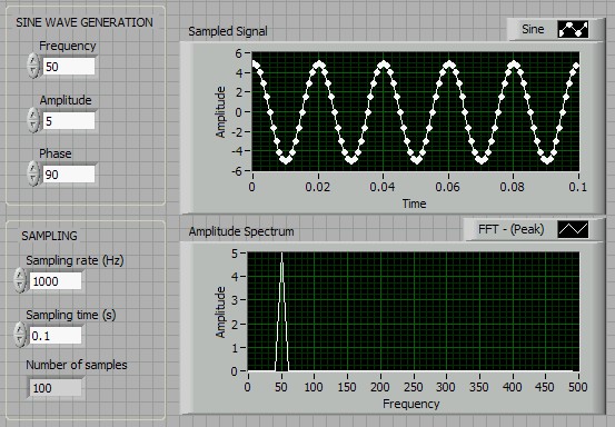
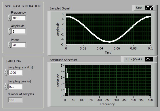
The default case, shown above, is a 50Hz sine wave with an amplitude of 5 and a phase of 90 degrees being sampled at 1000Hz for 0.1 seconds (100 samples). The actual points in the signal have been marked so it is clear where the samples are (you can easily change the plot format of a LabView graph by right clicking on it and selecting properties). The amplitude spectrum below shows exactly what it should - a value of 5 at a frequency of 50Hz. We have no aliasing problems because the signal frequency is well below the Nyquist, of 500Hz.

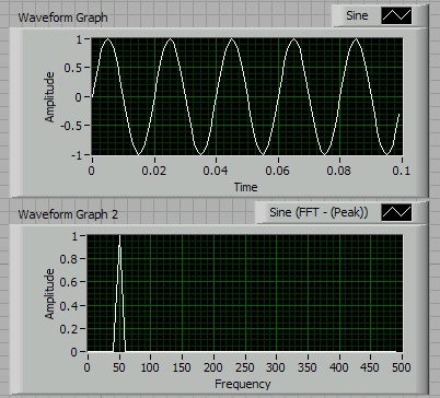
Press the 'Run Continuously' button (two nested arrows, just to the right of the run button) to repeatedly run the program, and click up on the frequency selector to increase the frequency to 130Hz. The signal should change accordingly (showing 13 wavelengths in the graph), and the spike in the amplitude spectrum should obediently move to the right, to 130Hz. Note that even though the spectrum is fine, the sampled signal is not quite as good as it was. This is because the higher we make the frequency the fewer samples are taken of each period of the wave.

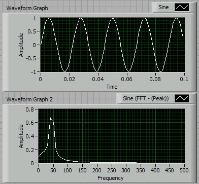
Continue increasing the frequency to 450Hz (the default frequency increment is 80Hz). The subjective quality of the sampled signal will continue to degrade, but the spectrum should remain fine. What happens now if we raise the signal to 530Hz, and then 610Hz, and so on. Try this. Instead of continuing to increase, the spectral peak starts coming back down.

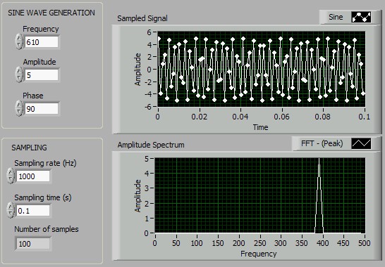
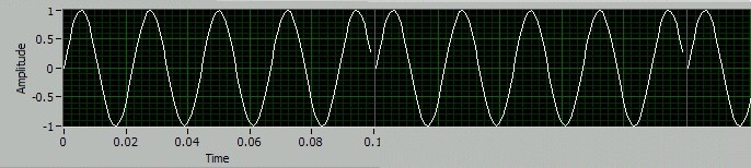
At 610Hz you should see a picture like that above, with a spike in the spectrum at 390Hz instead of 610. The reason is that, with less that two samples in every wavelength, samples of a high frequency signal look just like those from a low frequency one. You can see this very clearly if you go on increasing the signal frequency to 1010Hz. The time between each sample is almost equal to the period of the wave, so the samples show only a very slow variation, apparently at 10Hz.

In general aliasing creates two problems. First, it can cause us to mistake a high frequency signal for a low frequency one. This is common, for example, when electrical interference from a computer contaminates a sensor signal. The interference (usually a signal at many MHz) can get aliased and appear as though it is part of the legitimate low frequency sensor signal, and therefore be misinterpreted as a fluctuation in velocity, temperature, or  whatever physical property we are trying to measure. Second, when a signal contains a broad range of frequencies, aliasing can corrupt the entire shape of the spectrum. If, in our example above, we had used a broadband signal with energy at all frequencies from zero to 1010Hz in place of the sine wave, the spectral value at 610Hz would have got added to that at 390Hz, the value at 1010Hz would be added to that at 10Hz, and likewise at all other frequencies. We would have no way of separating these contributions and thus no way of extracting the true spectrum.

So how can we minimize the influence of aliasing on a spectral measurements? There are three measures we can take.

1. Take samples at a higher rate, so the Nyquist frequency exceeds the highest frequency in the signal. This is ideal, but not always possible since all A/Ds have maximum sampling rates. Also you may  not know what the highest frequency is. Signs that your sampling rate may be high enough are (i) that the spectral values you calculate at the highest frequencies are zero or almost zero (only works for broadband signals), or (ii) that spectra of the same signal measured at different sampling rates have the same shape. 

2. Use an analogue electrical filter to remove all the frequencies in the signal above the Nyquist before you sample it. (While you don't get the whole spectrum in this case, at least the part of the spectrum you do get is uncorrupted).

3. Be aware of the problem and alert to its possible presence. You may have to accept some minimal level of aliasing in your measurement. If you are aware that it is there, then you won't mis-interpret its effects.

5.2 Minimizing Broadening
Broadening of the spectrum describes what happens when a signal does not fit neatly into the measurement window. To see what this does we will use examples computed using the spectralDemo.vi introduced in section 4.2. The figure below shows (again) the output from this program in its default configuration (that shows an amplitude spectrum computed from 100 samples, taken at a rate of 1kHz, of a 50Hz sine wave with an amplitude of 1 and zero phase).

The spectrum looks perfect, but this is partly due to a lucky choice of parameters. The numerical Fourier transform treats the measured part of the signal as though it were part of an infinitely extending signal made up of repetitions of the measured part. At 50Hz exactly 5 periods of the wave fit into the measurement window between t=0 and 0.1s, so this measured part of the signal exactly fits to its copy from 0.1 to 0.2s which, in turn, fits to the copy from 0.2 to 0.3s, and so on. The implied infinitely extended signal is just a continuation of the 50Hz wave we measured, resulting in the perfect spectrum.

Of course this doesn't often happen in real life. The chances of picking a total measurement time that is an exact number of periods of the oscillation of a structure, or the flow rate in a fuel system are almost zero. Indeed, many signals we encounter in engineering measurement won't be periodic at all. So what happens in this case? Try re-running  spectralDemo.vi but with a signal frequency to 45Hz.

Now there is an extra half period at the end of the measurement window, so the implied repeated signal has a jumps at every repetition.

This rather ugly signal implies a range of frequencies (not just 45Hz) and the spectrum we get reflects exactly that. There is still a peak around 45Hz, but its amplitude is reduced and there are significant spectral levels over a whole range of surrounding frequencies. This is the problem of broadening.

Note that broadening doesn't affect signals that fall to zero at the ends of the measurement window (such as measurements from short duration phenomena like transients). Nor does it have much impact on signals where the amplitude spectrum varies smoothly from frequency to frequency, and there are no sharp spikes. However, when we have a signal containing one or more dominant frequencies (as in the present example) broadening can result in significant smoothing of the sharp spikes that would otherwise appear in the spectrum.

In this case the effects of broadening can be minimized by multiplying the signal by a smooth function that goes to zero or nearly zero at the ends of the record, called a window function. There are a variety of different commonly used window functions. Some are listed in the table below and illustrated in the following figure. All these have the form

where where T is the total record length and the constants c₀ , c₁ , and c₂ are as follows:

The Spectral Measurements VI includes the option of using any one of these (and other) window functions, or no window function at all. The window function can be selected (using the drop-down list under 'Window') in the dialog box displayed by double clicking on the VI. Changing to a Hanning window (probably the most widely used) for our current 45Hz example produces the effect shown below. The spectrum is not perfect, but much better than without a window function at all.

5.3 Dealing with Randomness
There are two kinds of randomness we have to deal with in measurements; unwanted noise that masks a sensor signal and thus the variations in the physical quantity we are trying to detect, or randomness in the physical quantity itself, such as in the velocity of a turbulent flow or in the unsteady lift of a stalling wing. Both of these situations call for averaging, but of different spectral quantities.

We can eliminate unwanted noise from a repeating signal by measuring multiple repetitions, and then averaging them together before taking the spectrum. As long as each repetition of the signal appears at the same position in the window each time we measure it, then the repeated signal will average to its true value, where as the random noise fluctuations will average to zero. The same result can be achieved by calculating the spectrum of each repetition, and then averaging the raw spectral coefficients a_n and b_n (before calculating amplitude and phase).

This exact situation is encountered when using computer data acquisition to measure the dynamic response of a structure. The response can be revealed for all frequencies, for example, by measuring the oscillations in time of the structure after it experiences an impulsive force (e.g. it is tapped with a hammer) and then calculating the spectrum (more about this later). There will be noise in the sensor not just from interference and electronics but also in the movement the structure picks up from other sources, such as building vibrations. So if the response is determined from a single measurement it will have uncertainties associated with this noise. Instead, the way to proceed is to repeat the measurement multiple times, triggering the data acquisition to start at the same instant (when the hammer hits, perhaps) each time, and then averaging the spectral coefficients. The more repetitions (averages) the lower the uncertainty in the spectrum will be.

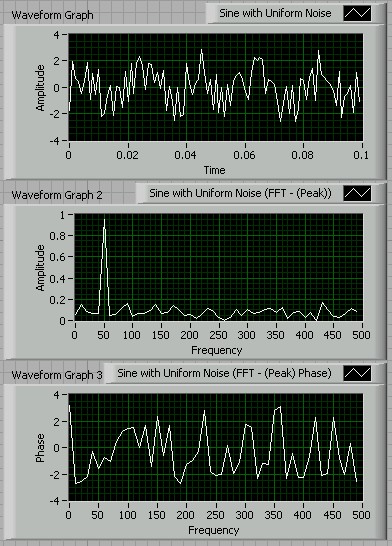
We can illustrate this process in LabView using the basic spectralDemo.vi program. After opening the program double click on the Simulate Signal VI and check the 'Add Noise' box. Note that 'Noise Type' should default to 'Uniform White Noise' with an amplitude of 0.6. Change the amplitude to 2.0. Run the program and your results should appear similar to that shown below.

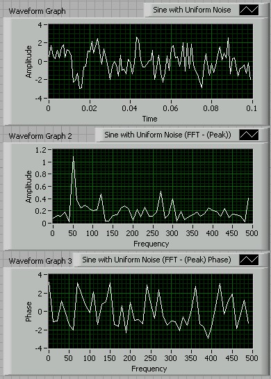
So much noise has been added that the original 50Hz sine wave is barely visible in the time trace. Even without averaging, however, the spectrum goes some way to separating that noise out - the amplitude spectrum still shows a clear peak at 50Hz. We can go much further though by averaging. Double click in the Spectral Measurements VI and check the 'Averaging' box.  Under 'Mode' choose 'Vector' (this ensures averaging of the coefficients a_n and b_n) and under 'Weighting' choose 'Linear' (just a regular average). Note that the 'Number of Averages' defaults to 10.

You can run the code at this point, but it won't take any averages. The problem is that the Spectral Measurements VI is expecting to receive 10 measured signals, and its only getting 1. To fix this, right click on an empty space in the block diagram, select 'Exec Ctrl' and then 'While Loop'. Click and drag a While loop surrounding all the program elements. When you release the mouse the loop will appear along with a 'Stop' button. We don't want this (we want the loop to stop when the averaging is done) so click on the stop button, and then hit delete. Finally connect the 'Averaging Done' output of the Spectral Measurements VI to the little stop sign left next to the while loop. Your final block diagram should appear as shown below.

Run the code (the 10 averages will whip by really fast), and you will see a dramatic reduction in the noise level in the spectrum. Note that the Simulate Signal VI always generates a sine wave with the same phase relative to the start of the measurement window, so there is no need to worry about triggering here.

Try running 100 averages, and see what it does to the noise level. If you have a hard time getting your code working, then you can download the one used to generate this figure, spectralNoise.vi.

Sometimes the random part of a signal is just as important as any deterministic part. The flow velocity in the wake of a circular cylinder high speed may often consist of a periodic fluctuation associated with vortex shedding, super-imposed on random turbulence. In this circumstance we will likely want to know the spectrum of the turbulence as much as we want to know that of the vortex shedding. Another example can be found in measuring the dynamic response of a structure. A second way to get the response at all frequencies is to measure the spectrum of the random movements produced by the structure in response to randomly fluctuating force (this technique will be discussed in more detail later).

To obtain the average spectrum of a signal with random components, we average the amplitude squared (A_n²) at each frequency, instead of the Fourier coefficients. This way the negative and positive fluctuations in the amplitude, produced by the randomness, don't cancel out. When the averaging is complete we can estimate the amplitude spectrum by taking the square root of these averages and the power spectrum as half these averages. Note that this type of averaging eliminates any phase information.

To demonstrate this type of averaging open spectralNoise.vi and double click on the Spectral Measurements VI and change the averaging mode to 'RMS'. Re run the code to produce a result like that below (for 10 averages).

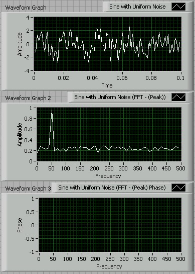
Note that the phase plot now just contains zeros (since there is no phase information). We see that the average noise amplitude (at each frequency) is about 20% of that of the sine wave, and that it has a flat spectrum. Incidentally, the term 'white' noise refers specifically to noise with a flat spectrum like this. Note that the more averages we take the smoother and more accurate the spectrum will become.

5.4 Exercises

1. A signal from a proximeter, used to sense the position of a beam structure, is being measured using an A/D converter and the spectrum calculated. The spectrum is calculated from a record of 1024 samples recorded at a rate of 100Hz. (a) What will be the lowest non-zero frequency in the spectrum? (b) What will be the highest? (c) What will the smallest difference in frequency that will be detectable in the spectrum? (d) What is the highest permissible frequency in the proximiter signal (in Hertz) if aliasing is to be avoided, and what name is given to this frequency? (e) If higher frequencies are present, what can be done to avoid corrupting the spectrum. Give two possible solutions.
2. For the situation in question 1: (a) Will a 40Hz sine wave signal from the proximeter be aliased? (b) Will a 40Hz square wave signal be aliased. To answer this, first run the code spectralDemo.vi to examine the frequency content of the square wave from 0 to 200Hz. Plot the results and then give your explanation.
3. The experiment outlined in question 1 proceeds, but the electrical system of a nearby wind tunnel generates interference in the proximeter signal at a frequency of 1580Hz. What frequency will this interference appear at in the spectrum? If you run the program spectralAliasing.vi to determine your answer, include the output plots with your solution.
4. At one stage in the experiment outlined in question 1, the proximeter is outputting a sine wave at 1.5Hz. (a) Determine how broadening effects this signal by running  spectralDemo.vi. Include output plots with your answer. (b) Choose a window function and regenerate the output plots. (c) How could the sampling scheme be modified to avoid broadening altogether?
5. Run the 45Hz sine-wave example of broadening for yourself. Record (by reading off the output graph) the amplitude indicated by the spectral peak. Then try, in turn, each of the different window functions available. Make a table of the peak amplitudes, as compared to the correct value of 1. Identify which window function is best by this measure, and which is worst.
6. Repeat the previous question for a 50Hz sine wave (that fits exactly in the window). Comment on the extent to which a window function might influence an otherwise perfect spectrum.
7. In each of the following cases identify whether the amplitude squared or the Fourier coefficients should be averaged to obtain a meaningful spectrum of the quantity indicated. Also indicate whether the data acquisition needs to be triggered, and what it should be triggered on. (a) The sound of the wind rushing past an aircraft cabin (or for that matter Randolph hall). (b) Vibrations in the hull of a ship (i) when we are interested in revealing the periodic vibrations due to the propeller, and (ii) when we are interested in revealing the stochastic response to the ocean waves. (c) Flexing of the a solar array powering a satellite produced by the impulsive heating experienced every time the satellite passes out of the Earth's shadow.
8. Load the program spectralNoise.vi. In its default state the code is set to average out the noise (vector averaging) accompanying a 50Hz sine wave. Change the type of result given by the Spectral Measurements VI to 'dB'. Run the code and show the results. Determine the difference in dB between the top of the residual noise in the spectrum and the 50Hz peak. Look at the definition of decibels and use this to ratio of noise amplitude at any frequency to signal amplitude. Increase the number of averages in steps (say to 30, 100, 300 and 1000), in each case noting the difference in dB and amplitude ratio. Can you discern a relationship in the results? If we wish to halve the noise level at any given condition, by how much do we need to increase the number of averages.
9. Load the program spectralNoise.vi. Change it so that it is set to determine the average spectrum of any random signals it generates, and increase the number of averages to 100. Check that the 'Results' are displayed in linear format, rather than dB, in the Spectral Measurements VI. Change the amplitude of the sine wave being generated to zero. Use the code to determine, and plot, average amplitude spectra for 'Gaussian White Noise', 'MLS Sequence' noise (a type of digital noise), and 'Inverse F Noise', by changing the options in the Simulate Signal VI (but otherwise retaining their default settings).  To what extent does the 'Inverse F Noise' have the spectral form implied by its name?

While many of the above spectral analysis examples consider single frequency signals, it is important to remember that the real power of spectral analysis is in extracting the frequency content of non-sinusoidal signals that contain many frequencies. Indeed when a frequency is known to be truly sinusoidal (a 'pure tone') then there are simpler techniques that can be used to determine that frequency and its amplitude and phase. In LabView, these techniques are encapsulated in the 'Tone measurements' VI. The following is one example of using this VI.

6.1 LabView Exercise

1. Write a simple code to generate test signals and do tone analysis on them:

   • Open a blank vi.

   • Right click on the empty block diagram and select 'Input' and then 'Simulate Sig'. This will add a VI that simulates the measurement of a signal.

   • Position the VI on the block diagram and a dialog box will open inviting you to set the characteristics of the measured signal. The default setting is for 100 samples at 1kHz of a 10.1Hz sine wave with an amplitude of 1 and phase of zero. Change the frequency to 50Hz and the phase to 45 degrees before clicking OK.

   • Right click on the block diagram and select 'Analysis' and then 'Tone'. Position this VI and an second dialog will open, asking you to pick the details of the tone analysis you want. Under 'Single Tone Measurements' make sure 'Amplitude', 'Frequency' and 'Phase' are all checked. .

   • Connect the 'Sine' output of the Simulate Signal VI to the 'Signals' input of the Tone Measurements VI. This completes the computational part of the code.

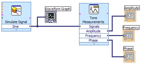
   • To plot some results, go to the front panel and add a graph, then return to the block diagram and connect the graph input to the 'Sine' output of the Simulate Signal VI, so as to display the signal.

   • To display the measured amplitude, phase and frequency, right-click on these outputs of the Tone Measurements VI and select 'Create>Numeric Indicator'. Arrange the indicators on the front panel - you may wish to drag out the phase indicator so it can display quite a long number. The reason here is that very small phases will be displayed in scientific notation, and the default size indicator clips the exponent of such numbers leading to a deceptive display. The block diagram of your completed code should look like that below.

2. Run the code and check it is working. Using the simulate signal VI try varying the amplitude, phase and frequency of the signal (choose odd values, like a phase of 23.23) to see how accurate the tone measurement is. Then complete the following exercises. The purpose of these exercises is to demonstrate how sensitive this method is to non-sinusoidal components, and noise.

   1. Set the amplitude, phase and frequency back to 1, 45 degrees and 50Hz respectively. Change the signal type to 'Square' and make sure the duty cycle (amount of time the square wave is high as a fraction of the total period) is set to 50%. Re-run the code, and note the amplitude, phase and frequency as compared with the actual values. Re-run the code for duty cycles of 30% and 10%, recording your measurements. Look over your results. What (if any) useful measurement does the Tone Measurements VI provide of these non-sinusoidal signals?

   2. Set the amplitude, phase and frequency back to 1, 45 degrees and 50Hz respectively, signal type to 'Sine' and 'Duty Cycle' to 50%. Check the 'Add noise' box and select 'Uniform White Noise' with an amplitude of 0.3. You will find that the noise introduces error into the tone measurements. Estimate the uncertainty in each of the measurements (amplitude,  phase and frequency) from twice their standard deviation. Take (and record) at least 5 values of these measurements to estimate the standard deviations.

1. spectralDemo.vi - Simulates measurement and Fourier transform of a single signal record, and presentation of the results as amplitude and phase spectra.
2. spectralAliasing.zip - Simulates the effects of aliasing on a measured signal and its spectrum. Two programs are included here; spectralAliasing.vi is the one to load and run, the other program (a subVI) needs to be unzipped into the same directory.
3. spectralNoise.vi - Demonstrates averaging of spectra to eliminate noise, or determine the spectrum of signals with random fluctuations